The data is stored in numpy format as a 2D matrix. The particular value represents the strain rate of a fiber optic cable located on a busy street (Jana Pawła II in Poznań). The data shows the passage of trams, trucks or cars along this street.
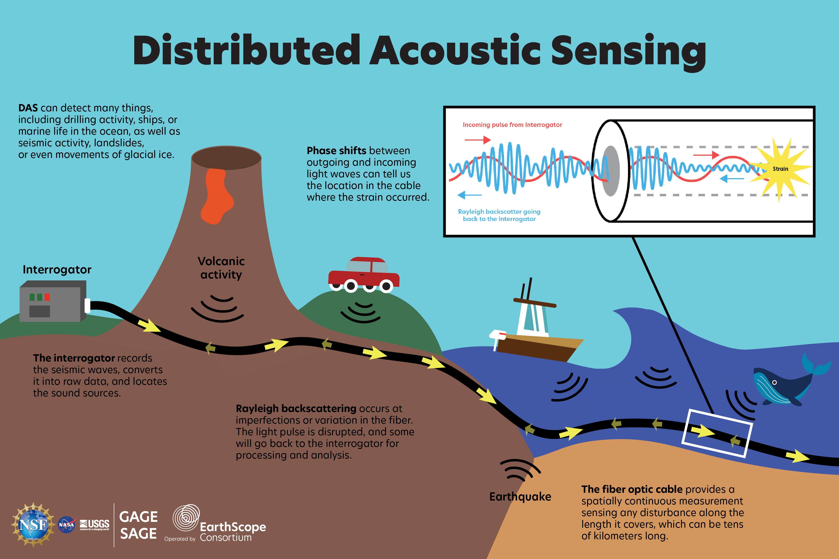
Distributed acoustic sensing (DAS) systems use fiber optic cables to provide distributed strain sensing. In DAS, the optical fiber cable becomes the sensing element and measurements are made, and in part processed, using an attached optoelectronic device. Such a system allows acoustic frequency strain signals to be detected over large distances and in harsh environments.


Load the raw Distributed Acoustic Sensing (DAS) measurements into memory as a time-space matrix, where rows represent time steps and columns represent fiber-optic spatial channels.
Convert the time-domain signal into the frequency domain to analyze dominant frequency content and enable frequency filtering.
Apply a band-pass frequency mask in the FFT domain to retain only frequencies associated with vehicle vibrations while suppressing noise.
Restrict the signal to the 5–40 Hz band where most vehicle-induced energy occurs, eliminating slow drift and high-frequency noise.
Transform the filtered frequency-domain signal back to the time domain using the inverse FFT.
Normalize each spatial channel independently to remove amplitude bias and take the absolute value to ensure all vibrations contribute positively.
Rescale the amplitude values so they fall within a consistent range (percenteils 3 and 99), enhancing contrast and making signals easier to visualize or threshold.
Convert the normalized signal into a binary image by keeping only values above a chosen percentile, isolating the strongest spatiotemporal features.
Reduce temporal resolution to decrease data size and computation while preserving enough detail to estimate vehicle speed.
After downsampling, the effective sampling rate becomes 6.25 Hz, which is sufficient to resolve vehicle speeds with ~1 km/h accuracy.
Convert filtered and resized data to an 8-bit grayscale image to visualize and process it using standard image-based algorithms.
Apply the Hough transform to detect straight-line patterns that represent vehicles traveling with near-constant speed along the fiber.
Use the Hough transform on the image-like data to identify strong linear patterns that correspond to moving vehicles.
Remove false or duplicate lines based on their position, slope, or speed consistency, keeping only meaningful vehicle tracks.
Scale detected line coordinates back to the original data’s time and spatial resolution so that speed calculations align with real-world distances.
Use the slope of each detected line (vehicle track) together with physical spacing dx and sampling interval dt to estimate vehicle speed in km/h.
Visualize the detected vehicle tracks and their computed speeds over the original DAS.


We can check how speed of the objects changed over time. For example speed plot for the first from the top detected object:

We decided to use the Straight Line Hough Transform algorithm for our project, recognizing both its advantages and limitations. It detects only straight lines from one end of image to another, so it won't detect artifacts that appear or disappear in the middle; But is it really a bad thing? After all no car just magically appears in the middle of the road, it had to travel whole path, optic fiber cable just didn't detect it. After testing a variety of preprocessing techniques - including morphological operations, blurring, high-pass filters etc - we found that simplicity was key. The preprocessing involved normalizing the DataFrame using two approaches: standardization and min-max scaling. We then adjusted the threshold percentile and performed binarization. The image was scaled appropriately to ensure compatibility with the Hough Transform algorithm. The results were satisfying: the algorithm successfully detected the majority of movements, with low number of false positives. However, the primary drawback of this approach is its inability to reliably detect shorter lines unless they are very close to the image boundaries. This limitation stems from the inherent properties of the Hough Transform, specifically the accumulator value, which is naturally lower for shorter lines. In conclusion, while the algorithm performs effectively for most cases, improving its sensitivity to shorter lines remains a challenge for future work.